


Document Actions
gvSIG-Desktop 1.10. User Manual
- Exporting layers
- Introduction
- Exporting a shape
- Exporting to dxf
- Exporting to postgis and Oracle Spatial
- Exporting to gml
- Exportar a kml
- Annotation layer
- Introduction
- Creating an annotation layer
- Editing an annotation layer
- Annotation layer properties
- Adding an annotation layer to the view
- Example of how to create an annotation layer
- Export to a raster layer
- Crear shape de geometrías derivadas
Exporting layers
Introduction
The “Export to...” tool allows you to save the elements selected in a layer in a different format. If no elements have been selected the whole layer will be exported. At the time of going to press the export formats supported by gvSIG were shape, dxf, and postgis and gml.
Exporting a shape
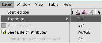
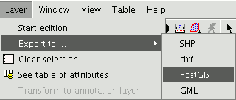
Select the “Layer” option from the menu bar then go to “Export to…/shp”.
If you have selected elements in the layer to be exported, gvSIG will tell you how many elements are going to be exported and will ask for confirmation before carrying out the operation.
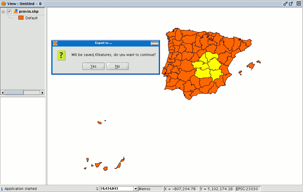
If you continue with the operation, a dialogue box will appear in which you will be asked to select the file the new shape is to be saved in.
When you have accepted, a new message will appear asking whether you wish to insert the new layer into the view.
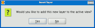
If you click on “Yes”, the layer will be added to the active view.
Exporting to dxf
Select the “Layer” option from the menu bar then go to “Export to…/dxf”.
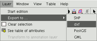
Follow the same process used for exporting to shape.
Exporting to postgis and Oracle Spatial
Select the “Layer” option from the menu bar then go to “Export to…/postgis”.
If you have selected any elements, a window will appear telling you how many elements are going to be exported (as in exporting to shp and dxf).
If you have selected any elements, a window will appear telling you how many elements are going to be exported (as in exporting to shp and dxf).
Remember that if the table already exists in the data base, the information it contains will be deleted.
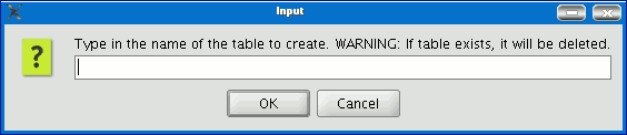
Write the name of the table and click on “Ok”. A new window appears in which you will have to input the parameters of the data base connection.
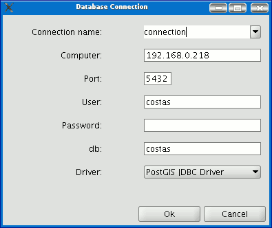
he parameters are:
Name: Name of the connection.
Computer: IP address of the computer the data base is hosted in
Port: Port on which the computer is listening to the postgreSQL service.
User: User name recognised by the administrator to make the connection
Password: User password required to validate the connection. db: The data base the new table is to be created in.
Driver: Driver required for the data base. (At the time of going to press, drivers for postGIS and mySQL were available). When you have input the connection parameters, click on “Ok”.
Exporting to gml
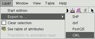
Select the “Layer” option from the menu bar then go to “Export to…/gml”.
Follow the same process used for exporting to shp or dxf.
Exportar a kml
From the menu bar, select Layer > Export to... > Keyhole Markup Language (KML).
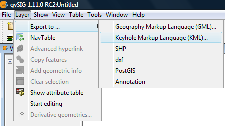
Layer menu, Export to KML
From here on the steps are exactly the same as for the Exporting to GML option.
Annotation layer
Introduction
This gvSIG tool makes advanced labelling easy.
The process creates a new layer which represents annotations.
The main features of this new layer can be summarised as follows:
- The new layer is only composed of the annotations created.
- The table associated with this new layer only contains the fields which refer to the text of the annotations (Text, Font, Colour, Height and Rotation).
- The layer created is always in .shp format, irrespective of the format of the original layer.
Creating an annotation layer
To create an annotation layer, first select the layer from the ToC (Table of Contents).
In the menu bar, select the “Layer” option, then select “Export to” and finally select the “Annotation” option.
This option opens the wizard which will guide you through the steps required to create the annotation layer.
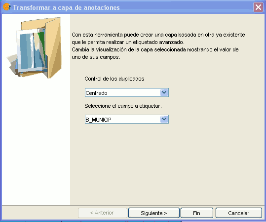
In the wizard’s first window, select the data which gvSIG requires to carry out the operation from the pull-down tab:
Duplicate control: Select either “None” or “Centred” to choose the position in which you wish the annotations to be inserted.
Centred: A label is created for each value and this will be inserted in the centre of all the labels which are the same.
None: A label is inserted for each value, even if these are repeated.
Select the field to be labelled: Choose the field which contains the text you wish the labels to show.
If you do not wish to modify the format of the annotations created by gvSIG and prefer a standard format, click on “Finish”. If you wish to customise the format, click on “Next”.
The wizard’s second window allows you to select the fields of attributes of a a table (if there are any) which contain the values which allow you to customise the labelling.
The following parameters can be customised.
Slope – the slope the annotation will have in the view.
Colour – annotation text colour.
Height – annotation text height.
Units – units in which the value assigned to the “Height” field are to be measured.
The options currently available are map units or pixels.
Font – annotation text font.
Set the values to be used for customising the required parameter (by pulling down the list).
Leave the default value in the fields you do not wish to customise.
Click on “Finish” when you have input these changes.
Editing an annotation layer
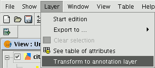
An annotation layer can be edited like any other layer. To start an editing session in gvSIG, select the layer in the Table of Contents and then select the option “Start edition”.
When you start an editing session, an option appears in the menu bar called “Modify annotation”. This will allow you to individually customise the annotation you wish to change.
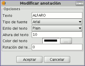
When you click on this button, the appearance of the cursor will change. You may graphically select the annotation by clicking on the point associated with the text and then access a set of properties shown in the following image.
Annotation layer properties
If we select the “Properties” option from the annotation layer contextual menu, the following box appears:
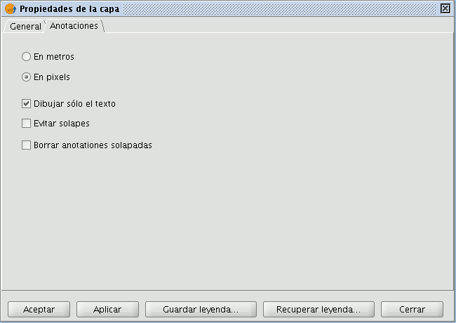
The “Layer properties” box has two tabs. The “General” tab allows you to access the general properties of the layer and the “Annotations” tab allows you to select: whether you wish the annotation text to be shown in pixels or metres in the view.
Whether you want only the text to appear (select the “Draw text only” option) or if you prefer the text to be accompanied by a location point (deselect the “Draw text only” option).
However, remember that this point is useful, for example, to move the annotation or to access the “Modify annotation” window.
If you wish to avoid overlays, activate the “Avoid overlays” option.
If you wish to eliminate overlaying annotations, activate the “Clear overlaying annotations” option.
Adding an annotation layer to the view
To add an annotation layer, click on the “Add layer” button in the tool bar

and select the “Annotation” tab.
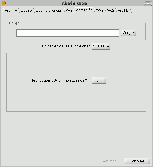
In the box you can select the annotation layer you wish to load, in addition to the units in which the annotations are displayed (pixels or metres) and the projection of the layer.
Example of how to create an annotation layer
The following image shows how an annotation layer is created out of a polygon layer called “muni10000.shp” which contains all the towns in the Valencian Region.
In the first window of the wizard, insert the type of duplicate control you wish to use and select the field which contains the text to be shown.
This is the field in a layer’s table of attributes which contains the name of the town.
If you do not wish to customise the presentation, click on “Finish” and indicate where you wish the new annotation layer to be saved.
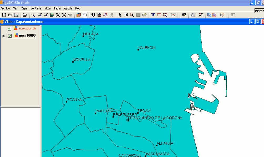
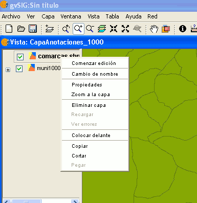
The following image shows the result (the rest of the fields in the wizard are left with their default values and this one is zoomed in) of creating the “annotation layer”.
The annotation layer which has been created is the one in red called “Towns” in the Table of Contents.
Export to a raster layer
This tool allows you to extract portions of a raster layer using a selection in the view or by inputting the coordinates that define the portion to be extracted.
It allows the user to change the spatial resolution of the clipping or of the whole image, choose the bands to be extracted or generate a new raster layer for each of the original bands.
To access this option, go to the ToC and select the raster layer you wish to select a portion of.
Then go to the Layer/Export to menu and select the “Raster” option.
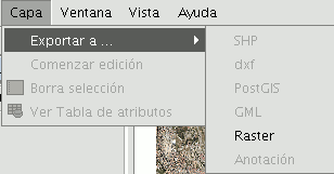
The following window appears:
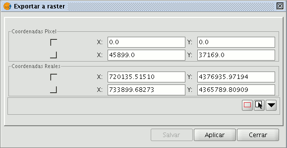
Image clipping
There are two ways of selecting an area to be clipped from the original raster layer:
You can use the text boxes in the window to input the data which correspond to:
- Real coordinates: If the source image is georeferenced.
- Pixel coordinates: If the source image is not georeferenced.
You can also make your selection directly from the view by clipping the whole image or selecting a part of it.
This button allows you to obtain a clipping from the whole image.
This button allows you to obtain a clipping from a selected area in the view. Place the cursor over the image, then click and drag. Check that the text boxes are automatically completed.
If you wish to save the raster layer clipping you have created, click on “Save” and select the location you wish to save this file in. The image will be saved in TIF format.

Changing spatial resolution
The controls that allow you to specify the clipping’s (or whole image) spatial resolution are located in the Clip table, with the additional options panel pulled down (to pull this panel down click on the button). You can define the resolution by specifying the Cell size or the Width and Height of the raster layer to be generated in pixels as well as choosing the interpolation method using the resolution change. At the moment, only the “Nearest neighbour” option is operational.

Band selection
The original raster layer’s band list appears at the bottom of the Clip table. You can use this list to choose the bands the output raster layer will have if you enable or disable the check boxes in the Bands column. If you check the Create one layer per band option, a new layer will be generated for each of the bands checked in the list. The new layers will be added to the ToC.
Saving and Adding a raster layer clipping to the current view.
When you have established all the parameters which define the raster layer clipping you have made, click on “Save”. This opens a dialogue box which allows you to search for a directory to save the clipping in. If you wish to add the layer to the view, go to the “Add layer” button in the tool bar once you have saved the clipping.
Example of a raster layer clipping
This example shows how a clipping is taken from an orthophoto.
First, select the area by defining a rectangle in the gvSIG view.
When you have finished, the coordinates will automatically be input into the text boxes based on the selection. You can fine tune these selected values from the view by inputting the new value directly into the text boxes containing the data.
Then pull down the box. As the resulting image is to be resampled, not as much resolution is required. Therefore, go to the “Spatial resolution” section and select “Width x Height”. This enables the text boxes so that you can input the output raster layer resolution.
When one value is input the other one is automatically completed when you press Enter or when you exit the field, as the proportions between the width and height must be maintained.
The cell size for the chosen output resolution is also calculated. If “Cell size” had been chosen, you would have had to specify the size in metres for each pixel and thus the width and height for the chosen cell size would have been calculated.
You now need to select the bands you want the output layer to have. In this case, select them all as this is a three-band orthophoto and we want to include them all.
Finally, for our example, the “Create a layer per band” option needs to be enabled to do just this.
Each new layer will have the same data type as the original image. If you click on “Save” a dialogue box opens to indicate the directory and image name.
To retrieve the layers you have created, go to the Add layer” button and then to the directory they were saved in.
Crear shape de geometrías derivadas
"New layer with derived geometries" tool.
This tool allows users to generate geometries derived from points or lines in a vector layer, and to store them as a new shape layer.
| Icon | Description |
|---|---|
 |
Derived geometries tool enabled if the TOC contains at least one visible point or line vector layer that is not in edit mode. |
 |
Derived geometries tool disabled if the TOC does not contain any visible point or line vector layers that are not in edit mode. |
The tool can be accessed from:
Via the menu: Layer / Derivative geometries
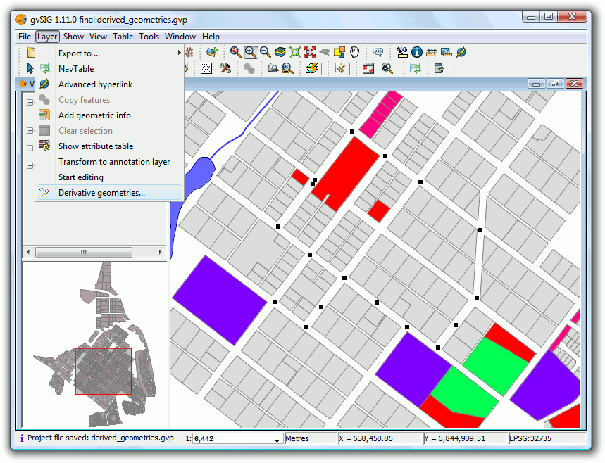
Menu path to the tool
Layer selection dialog and process
Upon choosing the tool a dialog for selecting layers is displayed:
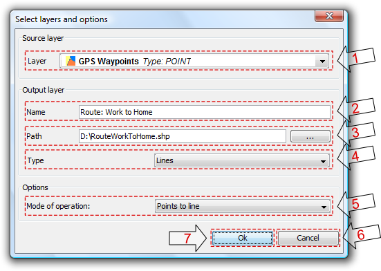
Selecting layers and process
- Source Layer: drop-down list of point or line vector layers in the current View that are not in edit mode. Select a layer to be the source layer.
- Name of the output layer: layer name that will appear in the TOC.
- Path of the output layer: full path for creating the new shapefile.
- Type of output layer: geometry type of the new layer. This depends on the type of process chosen (See options below).
- Type of process: select the type of geometry generation process. This depends on the geometry of the source layer. This process is applied to the source and destination layer pair until the tool is closed.
- Cancel: Close the tool.
- OK: Opens a control panel and displays data for the selected source layer. This control panel will be associated with source and output layers until it is cancelled.
| Source layer geometry type | Type of process | Target layer geometry type |
|---|---|---|
| Points | Points to line | Lines |
| Points | Points to polygon | Polygons |
| Lines | Close polylines | Polygons |
Process Control Panel
The control panel is associated with the layer and is shown every time the layer is activated in the TOC, as long as the layer is visible and not in edit mode.
The dialog has a semi-modal behavior in order to allow the user to continue working with gvSIG by using the minimize, maximize, resize and hide buttons (use the X, not the Cancel button, to hide the dialog).
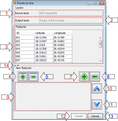
Process control panel
- Name of the source layer: Layer from the TOC that contains the source geometries.
- Name of the output layer: Name of the new derived geometry layer that will appear in the TOC.
- Table of features: Table showing the attributes of all the source layer's features. Source layer geometries selected in the View will also be selected in this table.
- Add all: Adds all the features of the source layer to the table of selected features.
- Remove all: Removes all features from the table of selected features.
- Enable snapping tool: Enables snapping tool on the source layer, without putting it into edit mode (only available in the Castilla y León extension for gvSIG 1.1.2).
- Add selected features: Adds only the selected features to the table.
- Remove selected features: Removes only the selected features from the table.
- Table of selected features: Table showing the attributes of all the features selected from the source layer. It has 2 extra columns:
- Order: Order to be used when generating the new geometry from the selected features in a point source layer, or when closing polylines in the case of a line source layer. The order can be changed with buttons 10 and 11.
- ID: Fixed ID number of the geometry in the vector layer.
- Move up: Moves the selected geometries up one position.
- Move down: Moves the selected geometries down one position.
- Create: Start the process of generating the derived geometries. If it doesn't already exist, a new layer is created, and the new geometries are added to this layer. The process is done in a thread, the progress of which is indicated by a progress bar.
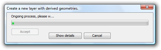
Progress bar
The results of the completed process can be viewed by clicking on the "View Details" button. There are three types of data that are of interest here:
- Number of geometries to create: depends on the geometry selected:
- If they are of type point: one line or polygon is created.
- If they are of type line: one polygon is created for each line.
- Number of geometries that could not be created: the subprocess failed, for example because a polygon couldn't be derived from simple lines that consist of only two points.
- Number of geometries created successfully: the new geometries created.
 This information is recorded in the gvSIG log.
The control panel is hidden during the process but becomes visible again when the progress dialog is closed.
- Cancel: Closes the control panel and de-registers the associated tools, thereby terminating the tool for the specified source layer.
- Expand / Collapse: Changes the position of the splitter, so as to display only the table of features, only the table of selected features and associated management controls, or both halves of the control panel interface.
Control Panel Behaviour
The control panel is linked to the source layer from the time it is created until it is cancelled by clicking the cancel button.
| Action | GUI Element | Description |
|---|---|---|
| Maximize |  |
Resizes the dialog so that it fills all available space. |
| Minimize |  |
Minimizes the control panel to a restore button. |
| Collapse |  |
Control panel is hidden but remains linked to both the source and output layers. Further operations between these layers can be performed once the panel is restored. |
| Resize | The size of the control panel can be increased or reduced by selecting and dragging the edge of the panel. | |
| Expand / Collapse splitter interface |  |
These controls are used to display only the table of source layer features, or only the table of selected features and associated management controls, or both halves of the control panel interface. |
| Cancel |  |
Closes the tool so that is no longer available for operations between the source and output layers. |
When the control panel is hidden it can be restored it by clicking on the source layer in the TOC.
If the View is closed when control panels are visible, the panels will be hidden and then restored when the View is reopened.
 Geometries derived from points do not retain any attribute values but do maintain the columns. Those derived from lines, keep all attributes.
Removing the new layer associated with control panel will result in the tool being ended and a warning being displayed to the user.
Examples
This example will show how to generate a line layer showing the path followed from home to work, and back again. The example uses the following four shape layers:
- Land-use: layer showing parcel boundaries of the town.
- Rivers: layer showing rivers in the town.
- Lakes: layer showing lakes in the town.
- GPS Waypoints: shape layer containing points recorded by a GPS on the drive to and from work. This layer will be used as the source layer in the example.
Once all four layers have been loaded the "Derived Geometries" tool can be selected and the following values entered:
- Source layer:
- Layer: GPS Waypoints
- Output Layer:
- Name: Route: Work to Home
- Path: .../RouteWorkToHome.shp
- Type: Lines
- Options:
- Mode of operation: points to line
When "OK" is clicked the new process control panel appears. If a file with the same name as the new output layer already exists then the user is asked whether to continue or not. If yes, then the file will be overwritten.
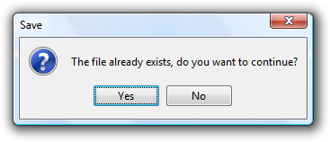
Warning of an existing layer
Minimizing the control panel will reveal the View:
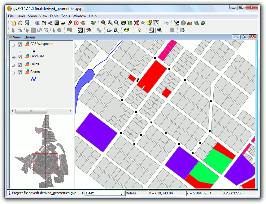
View showing the layers
The geometries can be selected from the top table in the control panel.
We select the first seven geometry points (1st route: work to home).
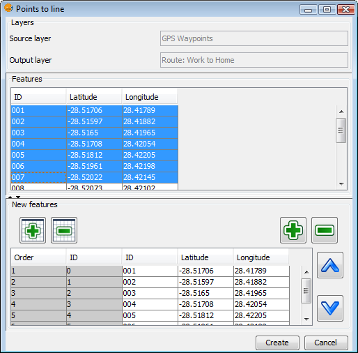
Selected geometries
Click "Create" to generate the first path:

Resulting route generated by the "Points to line" process
Modify the symbology so that the route stands out as a thick line.
To generate the route back, activate the control panel and select the remaining points from the source layer so that the line can be generated:
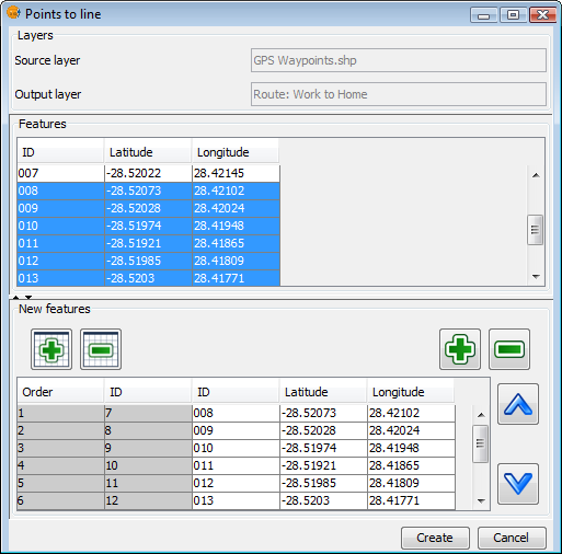
Selected geometries

Resulting new route
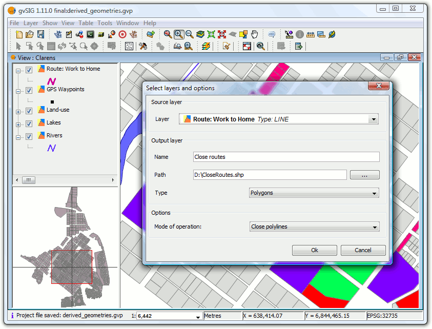
Finally suppose we are interested in the polygon formed by the closure of the routes.
Cancel the tool and then reopen it but this time use the new layer as the source:
- Source layer:
- Layer: Path: GPS Waypoints
- Output Layer:
- Name: Close routes
- Path: .../CloseRoutes.shp
- Type: Polylines
- Options:
- Mode of operation: close polylines
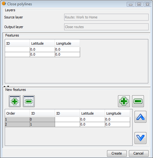
Process "close polylines"
Select all the geometries (the two polylines) and generate the polygons.
Selected geometries
Since the layer "Route: Work to Home" does not contain data due to the points to line process, we assign a distinguishing identifier to each by editing the layer.
Now apply some changes to the symbolology:
- Layer "Close routes": select a unique values symbology to distinguish the two polygons, and choose fill patterns that allow the lower layers to be seen.
- Layer "GPS Waypoints": Use a symbol of a car for the points and place the layer above the other layers.
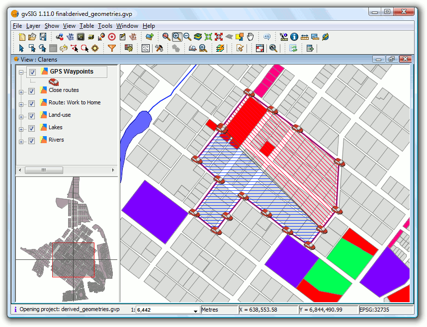
Results of the polygons generated by the "Close polylines" process


